
• From words to vectors: semantic proximity as an interface of understanding
Semantic Proximity
Table of Contents
- Context
- Concept explanation / theory
- Current applications and relevance
- Practical example: Kotlin + PGVector
- Limitations and debates
- Conclusion / synthesis
- Sources and recommended reading
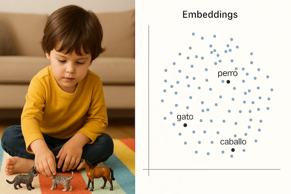
Before children learn to define concepts with precision, they can already group objects by “similarities”. A small child, when processing the sensory and symbolic information they receive, tends to place the dog and the cat in a nearby region within their interpretation of the world. That’s why they call them the same. It’s not exactly an error: we could consider it an early form of reasoning by similarity, a primitive intuition of what we now understand as semantic proximity.
In their longitudinal study, considered seminal in the field, Similarity, Specificity and Contrast (1986), Dromi and Fishelzon observed that children categorize the world not by fixed definitions, but by fuzzy similarity relationships. What artificial intelligence does today with vectors, the brain intuited from childhood: similar things are grouped together, even if they’re not named the same.
That intuition is now technology: semantic proximity allows modern systems to “understand” beyond literal text. This leap happened when language stopped being processed as plain text and began to be modeled as numerical vectors in high-dimensional spaces. Models like word2vec, GloVe, or BERT learned to represent meanings in coordinates, allowing mathematical operations to approximate semantic relationships. Thus, what was once fuzzy interpretation is now transformed into distance calculation. How is that modeled? How do we use it in real software?
Context
The concept of semantic similarity is not new. In computational linguistics, cooccurrence of terms and context analysis were already discussed in the 1950s. But then came several key leaps:
- word2vec (2013): allowed representing words as vectors that capture context similarities. Thanks to this, related concepts appear close in a vector space, even allowing operations like
king - man + woman ≈ queen. https://en.wikipedia.org/wiki/Word2vec - BERT and later models: took the idea further by generating vectors that depend on the context in which each word appears, allowing a more precise and nuanced understanding of language. https://en.wikipedia.org/wiki/BERT_(language_model)
This opened a new path: if meaning can be represented as a point in space, then the distance between points is a measure of similarity
Concept explanation / theory
Semantic proximity measures how close two elements are in a vector space trained to capture meanings. Some key principles:
- Embeddings: Numerical representation of words, phrases, or documents in an N-dimensional space.
- Distance metrics
- Semantic space: A space where “cat” is closer to “feline” than to “refrigerator”.
Example:
import kotlin.math.sqrt

fun main() {
    val cat = listOf(0.1, 0.3, 0.5)
    val dog = listOf(0.12, 0.1, 0.52)
    val cosSim = cosine(cat, dog)
    println(cosSim)
}

fun cosine(a: List<Double>, b: List<Double>): Double {
    val dotProduct = a.zip(b).sumOf { (x, y) -> x * y }
    val magnitudeA = sqrt(a.sumOf { it * it })
    val magnitudeB = sqrt(b.sumOf { it * it })

    return if (magnitudeA != 0.0 && magnitudeB != 0.0) {
        dotProduct / (magnitudeA * magnitudeB)
    } else {
        0.0
    }
}
A cosSim value close to 1 indicates high semantic similarity. The cosine metric is one of the most used to calculate this proximity because it measures the angle between two vectors, ignoring their magnitude. This is useful when what matters is the direction (i.e., the semantic pattern), not the intensity.
There are other possible metrics, such as Euclidean distance (which measures the linear distance between two points in space) or Manhattan distance (which sums the absolute differences in each dimension).
However, in high-dimensional spaces like those generated by embeddings, cosine tends to be more stable and representative: it penalizes long vectors less and tends to work better when data is normalized. That’s why it’s the default option in most semantic search systems.
Current applications and relevance
What is this useful for in modern software?
- Recommenders: showing content similar to what the user already saw.
- Semantic search: beyond exact keywords.
- Classification: identifying intentions or topics even without textual match.
- Knowledge graph: finding connections between ideas or concepts.
In backend development with Kotlin and PostgreSQL, we can use pgvector to store and query these vectors efficiently.
Practical example: Kotlin + PGVector
Suppose you have a text table and each entry has an embedding field of type vector(768). This size is not arbitrary: it corresponds to the embedding size generated by the nomic-embed-text model, which you can use to represent texts with a 768-dimensional numerical vector.
First we create the table and an HNSW index to optimize similarity search:
CREATE EXTENSION IF NOT EXISTS vector;
CREATE TABLE text (
   id UUID PRIMARY KEY,
   content TEXT,
   embedding vector(768)
);

CREATE INDEX idx_embeddings_hnsw_cosine
    ON text
    USING hnsw (embedding vector_cosine_ops);
The query in Kotlin using Spring Data JPA would be:
@Query(
    value = """
        SELECT content AS text,
	        1-(embedding <=> CAST(:embedding AS vector)) AS score
        FROM text
        ORDER BY embedding <=> CAST(:embedding AS vector) DESC
        LIMIT :limit
    """,
    nativeQuery = true,
)
fun findMostSimilar(
    @Param("embedding") embedding: String,
    @Param("limit") limit: Int = 5,
): List<Text>
Here we use the <=> operator from PGVector, which measures cosine similarity distance. It’s different from the <#> operator, which measures Euclidean distance. While <#> penalizes vector magnitude (linear distance), <=> focuses on direction, making it more suitable for comparing meanings.
You can see a complete example in this repository: github.com/apascualco/semantic-search
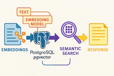
Flow diagram of a semantic search
Limitations
- Black-boxing: embeddings can capture model biases.
- Dimensionality: more dimensions ≠ better results.
- Updates: what happens if meanings or context change?
- Context vs. universal meaning: an embedding doesn’t always reflect the real intention of an ambiguous phrase.
Conclusion / synthesis
Semantic proximity is today the cornerstone of intelligent systems that understand, recommend, and connect. Its strength lies in converting language into geometry, and logic into distance. As developers, integrating this layer allows us to build products that “understand” beyond text.
Sources and recommended reading
- Mikolov et al. (2013). Efficient Estimation of Word Representations in Vector Space.
- pgvector: vector similarity search for Postgres
- The Illustrated Word2Vec
- Dromi, E. & Fishelzon, A. (1986). Similarity, Specificity and Contrast